How To Add Alternate Row Color In Excel

How to Add Alternate Row Color in Excel?

Below mentioned are the two different methods to add color to alternative rows:

Now, let the states talk over each method in particular with an case.

The quickest and near straightforward approach to use row shading in Excel is by utilizing predefined.

First, nosotros must select the data or range where we want to add together the colour in a row.
So, click on the "Insert" tab on the Excel ribbon and click "Table" to choose the function.
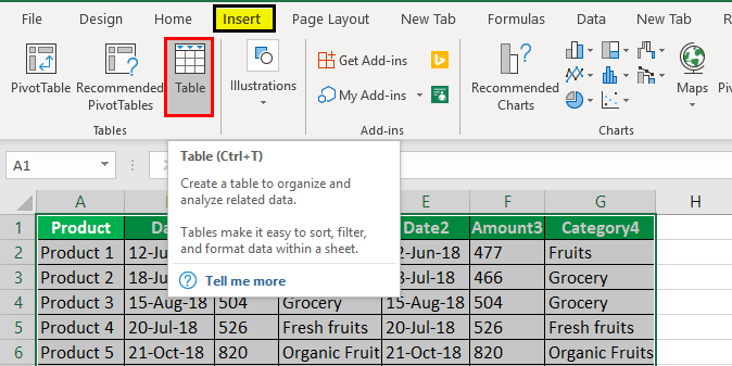
When we click on the "Tabular array," the dialog box will select the range.
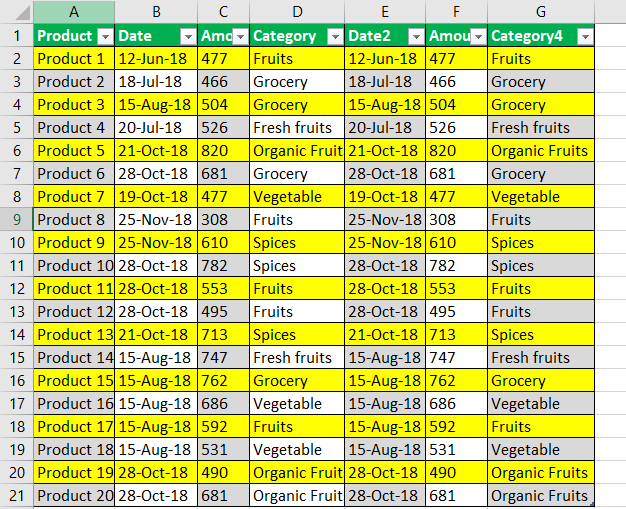
Click on the "OK." Now, we will get the table with alternating row colors in Excel, every bit shown below:
Suppose we do not want the table with rows. We would preferably have alternate column shading but without the table usefulness. We can undoubtedly modify over the table back to a standard range. Nosotros need to select whatsoever cell inside the table, right-click and choose "Convert to Range" from the setting menu.
Then, select the tabular array or data, and get to the "Design" tab.
Next, we need to go to table style and choose the colour of the table which is required and selected by us.

Stride 1: First, we need to select the data or range in the Excel sail.
Step ii: Get to the "Home" tab and "Styles" group, and click on conditional formatting in the Excel Provisional formatting is a technique in Excel that allows us to format cells in a worksheet based on certain conditions. It can be found in the styles section of the Home tab. read more than ribbon.

Step three: Choose a "New Rule" from the drop-down list in excel A driblet-downwardly list in excel is a pre-defined list of inputs that allows users to select an option. read more :

Step 4: In the "New Formatting Rule" dialog box, we must choose the option at the bottom of the dialog box, "Use a formula to determine which cells to format," and insert the following formula in a tab to get the result
=MOD(ROW(),two)=0

Step five: Click the "Format" button on the right-manus side, click on the switch to the "Fill" tab, and cull the groundwork color we want to use or required for the banded rows in the Excel sheet.

Footstep 6: In the dialog box, equally shown higher up, the colour we have selected will appear under the "Sample" at the bottom of the dialog box. If nosotros are satisfied with the color, click "OK" to cull the same colour, which shows in a sample.
Step seven: One time we click on "OK," it will carry us back to the "New Formatting Dominion" window in the Excel canvas, and when yous click "OK" again, apply the Excel color to the alternate row of the certain rows. Click "OK." We will get the alternate row color in Excel with yellow color, as shown beneath.

To meliorate the readability of the Excel sail, some users shade every other row in a huge Excel sheet.
Colors can enable u.s. to envision our information adequately by empowering us to perceive gatherings of related data by sight.
When we use the color in your spreadsheet, this theory makes the difference.
Calculation shading to alternating rows or columns (which is chosen shading banding) can brand the information in our worksheet less demanding to examine.
If any rows are inserted or deleted from the row shading, it automatically adjusts to maintain our tabular array's pattern.

Nosotros must always use decent colors while coloring the alternate color considering the vivid color cannot solve our purpose.
While using the conditional formula, we must e'er enter the formula in the tab. Otherwise, we will non be able to colour the row.
We should employ nighttime colors for the text to hands read the data in the Excel worksheet.
If we desire to impress your excel canvass The print feature in excel is used to print a sheet or any data. While nosotros can print the entire worksheet at one time, we likewise have the option of printing only a portion of it or a specific table. read more , we must ensure that we use a lite or decent colour shade to highlight the rows to read information technology very hands.
We must attempt non to use the excess conditional formatting function in our information because it creates defoliation.

Source: https://www.wallstreetmojo.com/excel-alternate-row-color/